Behind the maps
Data Source
All data on the interactive maps are sourced from the CORDEX-CORE framework, a standardization for regional climate model output. We currently use the REMO2015 and REGCM4 regional climate models. REMO2015 and REGCM4 are the only two RCMs that have been run on all domains in CORDEX-CORE, an effort which downscales data from multiple GCMs in the CMIP5 ensemble of global climate models. We will continue to consider additional models for inclusion as they become available.
Days over 32°C (90°F) at 1°C of warming
-
0
-
1-7
-
8-30
-
31-90
-
91-180
-
181-365
These two maps depict the difference in data resolution between General Circulation Models (GCMs), and Regional Climate Models (RCMs). Most GCMs have a grid cell size of approximately 250km on a side. RCMs use GCM data as an input and then downscale that data using regionally-specific dynamics. This results in model output with a higher resolution. RCM grid cells commonly range from 10 to 50km on a side. Data source: CMIP5, Cordex-Core, REMO2015 and RegCM4. Processed by Woodwell Climate Research Center.
Geographic coverage
- One of the first things you might notice is the lack of data over the Arctic, Antarctica, and all oceans for most Probable Futures maps. CORDEX-CORE does not include output covering the Arctic, Antarctica, and some islands. Additionally, we chose not to display data over oceans to increase efficiency on the “back end” of the maps, and to improve the user experience. In rare cases, we have removed data in individual cells due to anomalies in model output or geographic coverage. In our drought maps, we have chosen to omit data over deserts, as they are dry year-round.
Map style
- Every two-dimensional representation of our spherical Earth is going to suffer from distortions. There are maps that do a better job of minimizing distortions, such as the Equal Earth Projection. When we present static maps, we often employ Equal Earth. For the interactive maps we use the Mercator Projection. This projection makes the spherical earth a rectangle by forcing the curved longitudinal lines straight up and down. The resulting distortion portrays areas far away from the equator as much larger than they actually are. For example, Greenland and South America appear to be roughly the same size. In fact, South America is about 8 times larger than Greenland. We also have a globe view available in the interactive maps.
Warming scenarios
- Baselines are important to have as a reference point for the past, and to understand the scale and rate of change as the planet warms. A standard baseline time period in climate science and international climate policy is 1850-1900. This range is often called “pre-industrial temperature”. The “warming scenarios” of 0.5, 1, 1.5, 2, 2.5, or 3°C represent global average temperatures relative to the pre-industrial average.
- Probable Futures uses CORDEX-CORE data, which is available for 1970–2100. Since 1971–2000 had a global mean surface temperature of 0.5°C above pre-industrial temperatures, that time period is a good baseline for our maps.
- Each warming scenario above 0.5°C represents a twenty-one-year time span. There are a couple of reasons to take data from several years on either side of a specific scenario. First, it provides a range of temperatures around each threshold. This range is valuable because even when the climate is “at” a certain average temperature, there will be variations around that average, e.g., warmer and colder years. Second, powerful phenomena that happen regularly but not annually, most notably El Niño and La Niña, tend to occur every 2 to 7 years and can last less than a year or multiple years. By including 10 years on either side of the threshold year, our results will include some El Niño and La Niña events from each of the underlying models.
Grid cells
- The data behind Probable Futures maps are represented in 22-kilometer squares called “grid cells.” Most grid cells show three values that help summarize the distribution of model simulations within that cell. The mean value is averaged across the entire distribution. The median is the midpoint of the distribution, meaning half of the outcomes are either above or below this number. The median represents the outcome that we would most expect to see over time at that level of warming. The 5th and 95th percentile values can be thought of as infrequent outcomes that provide a sense of the range of possible outcomes. It is important to emphasize that the range of possible outcomes extends beyond those values. For example, 5% of the values in the simulated years have values lower (higher) than the 5th (95th) percentile value shown. Extreme outcomes that can have enormous impacts lie beyond the 5th and 95th percentile values.
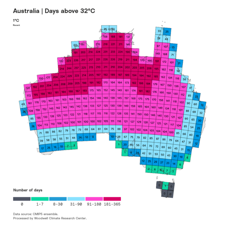
This map of Australia displays the grid cell methodology used in climate models to project localized conditions. The continent of Australia is divided into grid cells that are 250 kilometers to a side, each displaying the average of the distribution of values behind each cell. In other words, the models project many different outcomes for “days above 32°C” in each cell. What you see here is the average of those outcomes for each cell at 1°C of warming.
- The models calculate average conditions across each 22-square-kilometer area. For example, if one grid cell covers part of a mountain and an adjacent valley, or straddles both land and ocean, the value of that grid cell represents the average of those two different climate conditions.
- Think of the specific values in each grid cell not as precise, but as indicating direction and magnitude of change. Natural climate variability will occur in any given year, and outcomes may be higher or lower than the average, including the possibility of extreme events beyond the ranges portrayed on the maps. Extreme events are critical when considering climate change, but climate models are better at simulating averages than extremes.
Key
- The key is located in the bottom left-hand corner of each map. It explains the relationship between the values in the data and the colors on the map.
- The colors on Probable Futures’s maps are not colors you might expect to represent climate phenomena like heat or precipitation. This choice was intentional. First, we do not want to send subtle signals to the user about what color is “good” or “bad.” Each of us brings connotations and biases when looking at a map and associates different colors with different ideas and feelings. We chose colors that don’t easily correspond to common biases. Second, we chose colors that would work well for many people who have difficulty seeing colors. Third, we sought color combinations that would allow the viewer to see distinctions and change. We hope the color palette will encourage you to look closely and read the supporting resources to better understand the data.
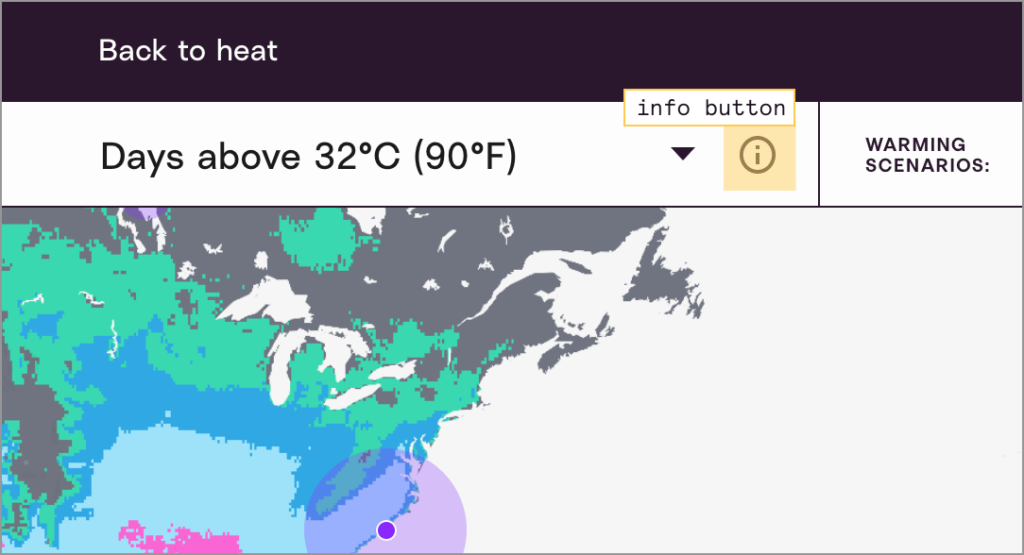
- Every map features an info button next to the drop-down box of maps. This button provides context and methodology for the specific dataset behind each map.
Navigate
- We encourage you to start with a global view. Our climate is a global system, and the weather in any location connects to the rest of the system. Similarly, we live in a globalized world, and the impacts of climate change in a given region are likely to have ramifications elsewhere.
- Next, zoom down to a large region, perhaps one you are familiar with. Move through the warming scenarios and observe how the trends relate to topography, proximity to bodies of water, and other natural features.
- Then, click on a cell to understand the distribution of values behind it. Perhaps do the same for surrounding cells and observe how similar or different they are, and what might influence those differences. Few people have ever experienced rainforests or tundra, but we encourage you to examine changes in those areas because they are vital to the stability of our climate.
Consider
- We can divide Earth up into patterns of temperature and precipitation called climate zones. For example, places may be far from one another but have very similar climate conditions (e.g., Northern California, coastal Australia, and parts of South Africa). In contrast, two locations might be very close on the map, but a mountain range might divide them. In such a case, a tropical zone might be right next to a desert zone. These climate zones were stable for over 10,000 years, but they are already shifting. Climate change will continue to shift patterns of temperature and weather, as warmer conditions move north from the equator. Consider what might happen as local climates change fundamentally. Think about how climate change will challenge plants, animals, infrastructure, and agriculture and how plants, animals and humans might adapt or migrate.
- From one region to the next, climate may differ dramatically depending on topography and other factors. However, it is important to consider that regions are highly integrated, often sharing populations, infrastructure, government, economic interdependencies, and other connections. Changes that appear for any region on Probable Futures maps will have impacts beyond their given area.
Imagine
- As you explore, consider factors in society that have duration—or that rely on long-term planning, such as a school, house, or farm, or an obligation such as a mortgage or treaty. Then, imagine the ways that climate change could directly or indirectly affect those things.
- You might also think in terms of thresholds. Human health has survivability thresholds, infrastructure like roads or the electrical grid has engineering thresholds, ecosystems contain crucial disturbance thresholds. Many of these thresholds are specific to a certain community or region, and the best people to consider those thresholds will be people with local knowledge.
- We hope that spending time with Probable Futures will encourage you to reach out to people around you, including people responsible for, and with expertise in, health, ecology, infrastructure, and government. Strengthening community is perhaps the best form of climate preparedness.